Temperature-pressure (T-p) Profiles#
The T-p profile describes the thermal structure of an atmosphere as a function of pressure.
For retreival models, typically a quick to calculate, physically plausible parameterised T-p profile that forms the basis for the forward radiative-transfer model.
Exo Skryer provides several analytical T-p profile functions in the vert_Tp module.
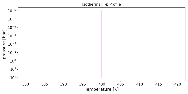
Isothermal#
The simplest T-p profile is assuming that the entire atmosphere is a constant value:
This is particularly useful for transmission spectroscopy. For emission, do not use an isothermal atmosphere unless under very specific test conditions, as no spectral features would be produced.
Required parameters: \(T_{\rm iso}\) [K]
Example Plot:
import numpy as np
import matplotlib.pyplot as plt
from exo_skryer.vert_Tp import isothermal
from exo_skryer.data_constants import bar

# Create pressure grid
nlev = 100
p_bot = np.log10(100.0)
p_top = np.log10(1e-6)
p_lev = np.logspace(p_bot, p_top, nlev) * bar  # 1e-6 to 100 bar in dyne/cm²

# Example parameters
params = {"T_iso": 400.0}
T_lev, T_lay = isothermal(p_lev, params)

# Plot
fig, ax = plt.subplots(figsize=(10, 5))
ax.semilogy(T_lev, p_lev/bar, c='orchid')
ax.set_xlabel('Temperature [K]', fontsize=16)
ax.set_ylabel('pressure [bar]', fontsize=16)
ax.set_title('Isothermal T-p Profile', fontsize=14)
ax.tick_params(labelsize=14)
ax.invert_yaxis()
plt.tight_layout()
(Source code, png, hires.png, pdf, svg)

Example YAML Configuration:
physics:
  vert_Tp: isothermal

params:
  - { name: T_iso, dist: uniform, low: 500.0, high: 2000.0, transform: logit, init: 1000.0 }
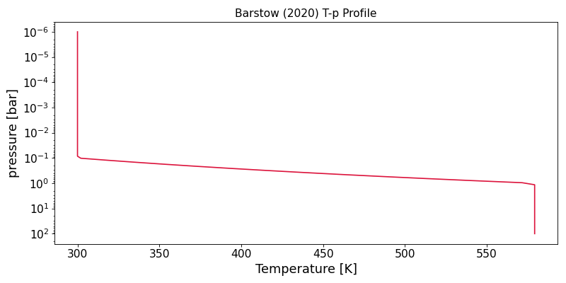
Barstow (2020)#
Barstow (2020) used a simple T-p stucture with the following form:
where \(p_1\) = 0.1 bar, \(p_2\) = 1.0 bar and \(\kappa\) is the adiabatic coefficient (default = 2/7). This forms an initial upper atmosphere isotherm at \(T_{\rm strat}\) at \(p \le p_1\), an adiabatic gradient for \(p_1 < p < p_2\), then a deep isothermal region at \(p \ge p_2\).
Required parameters: \(T_{\rm strat}\) [K]
import numpy as np
import matplotlib.pyplot as plt
from exo_skryer.vert_Tp import Barstow
from exo_skryer.data_constants import bar

# Create pressure grid
nlev = 100
p_bot = np.log10(100.0)
p_top = np.log10(1e-6)
p_lev = np.logspace(p_bot, p_top, nlev) * bar

# Example parameters
params = {"T_strat": 300.0}
T_lev, T_lay = Barstow(p_lev, params)

# Plot
fig, ax = plt.subplots(figsize=(10, 5))
ax.semilogy(T_lev, p_lev/bar, c='crimson')
ax.set_xlabel('Temperature [K]', fontsize=16)
ax.set_ylabel('pressure [bar]', fontsize=16)
ax.set_title('Barstow (2020) T-p Profile', fontsize=14)
ax.tick_params(labelsize=14)
ax.invert_yaxis()
plt.tight_layout()
(Source code, png, hires.png, pdf, svg)

Example YAML Configuration:
physics:
  vert_Tp: Barstow

params:
  - { name: T_strat, dist: uniform, low: 100.0, high: 1000.0, transform: logit, init: 300.0 }
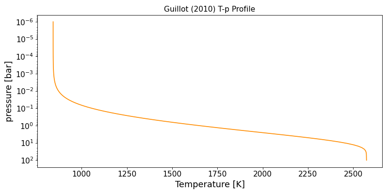
Guillot (2010)#
The Guillot (2010) analytic semi-grey radiative-equilibrium profile combines internal heating and external irradiation, commonly used for hot Jupiters and other irradiated planets.
Required parameters: \(T_{\rm int}\) [K], \(T_{\rm eq}\) [K], \(\log_{10} \kappa_{\rm ir}\) [cm2 g-1], \(\log_{10} \gamma_v\) (visible-to-IR opacity ratio), \(\log_{10}g\) [cm s-2], \(f_{\rm hem}\) (hemispheric redistribution factor)
import numpy as np
import matplotlib.pyplot as plt
from exo_skryer.vert_Tp import Guillot
from exo_skryer.data_constants import bar

# Create pressure grid
nlev = 100
p_bot = np.log10(100.0)
p_top = np.log10(1e-6)
p_lev = np.logspace(p_bot, p_top, nlev) * bar

# Example parameters for a hot Jupiter
params = {
    "T_int": 100.0,
    "T_eq": 1000.0,
    "log_10_k_ir": -2.0,
    "log_10_gam_v": -2,
    "log_10_g": 3.0,
    "f_hem": 0.25
}
T_lev, T_lay = Guillot(p_lev, params)

# Plot
fig, ax = plt.subplots(figsize=(10, 5))
ax.semilogy(T_lev, p_lev/bar, c='darkorange')
ax.set_xlabel('Temperature [K]', fontsize=16)
ax.set_ylabel('pressure [bar]', fontsize=16)
ax.set_title('Guillot (2010) T-p Profile', fontsize=14)
ax.tick_params(labelsize=14)
ax.invert_yaxis()
plt.tight_layout()
(Source code, png, hires.png, pdf, svg)
YAML Configuration:
physics:
  vert_Tp: Guillot

params:
  - { name: T_int, dist: uniform, low: 100.0, high: 1000.0, transform: logit, init: 500.0 }
  - { name: T_eq, dist: uniform, low: 1000.0, high: 3000.0, transform: logit, init: 1500.0 }
  - { name: log_10_k_ir, dist: uniform, low: -6, high: 6, transform: logit, init: -2 }
  - { name: log_10_gam_v, dist: uniform, low: -3, high: 3, transform: logit, init: 0.0 }
  - { name: log_10_g, dist: uniform, low: 2.0, high: 4.0, transform: logit, init: 3.0 }
  - { name: f_hem, dist: delta, value: 0.25, transform: identity, init: 0.25}
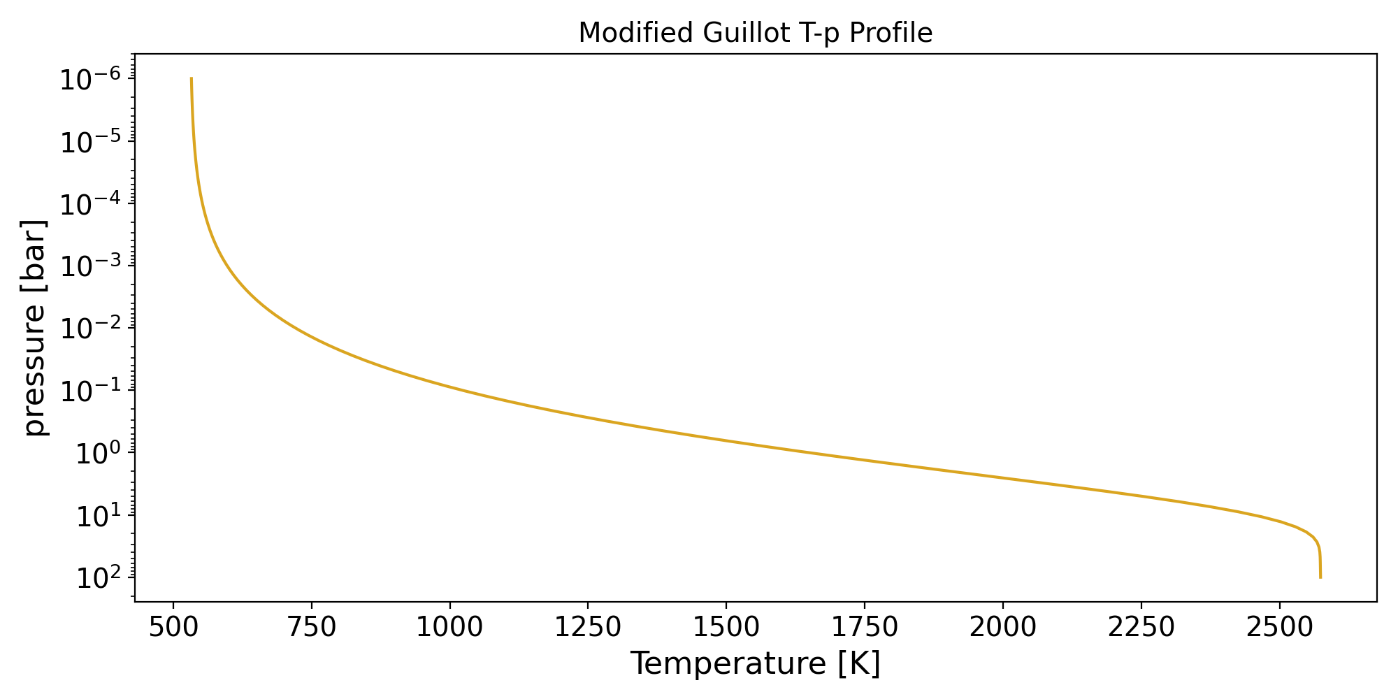
Modified Guillot#
The modified Guillot profile generalises Guillot (2010) by replacing the fixed irradiated Hopf term with a stretched-exponential transition in pressure. This reduces the strict upper-atmosphere isothermal tendency while retaining the deep-atmosphere semi-grey behavior.
with \(\tau = (\kappa_{\rm ir}/g)\,p\). In the current implementation, \(q_{\rm int}=2/3\) is fixed.
Required parameters: \(T_{\rm int}\) [K], \(T_{\rm eq}\) [K], \(\log_{10}\kappa_{\rm ir}\) [cm2 g-1], \(\log_{10}\gamma_v\), \(\log_{10}g\) [cm s-2], \(f_{\rm hem}\), \(q_{{\rm irr},0}\), \(\log_{10}p_t\) [bar], \(\beta\)
import numpy as np
import matplotlib.pyplot as plt
from exo_skryer.vert_Tp import Modified_Guillot
from exo_skryer.data_constants import bar

# Create pressure grid
nlev = 100
p_bot = np.log10(100.0)
p_top = np.log10(1e-6)
p_lev = np.logspace(p_bot, p_top, nlev) * bar

# Example parameters
params = {
    "T_int": 100.0,
    "T_eq": 1000.0,
    "log_10_k_ir": -2.0,
    "log_10_gam_v": -2.0,
    "log_10_g": 3.0,
    "f_hem": 0.25,
    "q_irr_0": 0.1,
    "log_10_p_t": -1.0,
    "beta": 0.5
}
T_lev, T_lay = Modified_Guillot(p_lev, params)

# Plot
fig, ax = plt.subplots(figsize=(10, 5))
ax.semilogy(T_lev, p_lev/bar, c='goldenrod')
ax.set_xlabel('Temperature [K]', fontsize=16)
ax.set_ylabel('pressure [bar]', fontsize=16)
ax.set_title('Modified Guillot T-p Profile', fontsize=14)
ax.tick_params(labelsize=14)
ax.invert_yaxis()
plt.tight_layout()
(Source code, png, hires.png, pdf, svg)
YAML Configuration:
physics:
  vert_Tp: modified_guillot

params:
  - { name: T_int, dist: uniform, low: 100.0, high: 1000.0, transform: logit, init: 500.0 }
  - { name: T_eq, dist: uniform, low: 1000.0, high: 3000.0, transform: logit, init: 1500.0 }
  - { name: log_10_k_ir, dist: uniform, low: -6, high: 6, transform: logit, init: -2.0 }
  - { name: log_10_gam_v, dist: uniform, low: -3, high: 3, transform: logit, init: 0.0 }
  - { name: log_10_g, dist: uniform, low: 2.0, high: 4.0, transform: logit, init: 3.0 }
  - { name: f_hem, dist: delta, value: 0.25, transform: identity, init: 0.25 }
  - { name: q_irr_0, dist: uniform, low: 0.01, high: 1.0, transform: logit, init: 0.3 }
  - { name: log_10_p_t, dist: uniform, low: -8.0, high: 2.0, transform: logit, init: -2.0 }
  - { name: beta, dist: uniform, low: 0.1, high: 1.0, transform: logit, init: 0.5 }
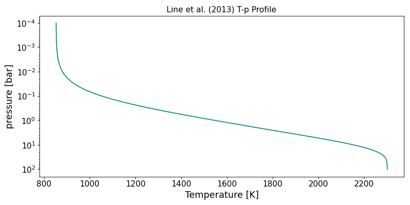
Line (2013)#
The Line et al. (2013) profile extends the Guillot framework with two visible opacity channels, allowing for flexible thermal inversions or more complex T-p constructions.
Required parameters: \(T_{\rm int}\) [K], \(T_{\rm eq}\) [K], \(\log_{10} \kappa_{\rm ir}\) [cm2 g-1], \(\log_{10}\gamma_{v1}\), \(\log_{10}\gamma_{v2}\), \(\log_{10}g\) [cm s-2], \(f_{\rm hem}\), \(\alpha\)
import numpy as np
import matplotlib.pyplot as plt
from exo_skryer.vert_Tp import Line
from exo_skryer.data_constants import bar

# Create pressure grid
nlev = 100
p_bot = np.log10(100.0)
p_top = np.log10(1e-4)
p_lev = np.logspace(p_bot, p_top, nlev) * bar

# Example parameters
params = {
    "T_int": 100.0,
    "T_eq": 1000.0,
    "log_10_k_ir": -2.0,
    "log_10_gam_v1": -2.0,
    "log_10_gam_v2": -1.0,
    "log_10_g": 3.0,
    "f_hem": 0.25,
    "alpha": 0.5
}
T_lev, T_lay = Line(p_lev, params)

# Plot
fig, ax = plt.subplots(figsize=(10, 5))
ax.semilogy(T_lev, p_lev/bar, c='teal')
ax.set_xlabel('Temperature [K]', fontsize=16)
ax.set_ylabel('pressure [bar]', fontsize=16)
ax.set_title('Line et al. (2013) T-p Profile', fontsize=14)
ax.tick_params(labelsize=14)
ax.invert_yaxis()
plt.tight_layout()
(Source code, png, hires.png, pdf, svg)

YAML Configuration:
physics:
  vert_Tp: Line

params:
  - { name: T_int, dist: uniform, low: 100.0, high: 1000.0, transform: logit, init: 500.0 }
  - { name: T_eq, dist: uniform, low: 500.0, high: 3000.0, transform: logit, init: 1500.0 }
  - { name: log_10_k_ir, dist: uniform, low: -6, high: 6, transform: logit, init: -2 }
  - { name: log_10_gam_v1, dist: uniform, low: -3, high: 3, transform: logit, init: -2.0 }
  - { name: log_10_gam_v2, dist: uniform, low: -3, high: 3, transform: logit, init: -1.0 }
  - { name: log_10_g, dist: uniform, low: 2.0, high: 4.0, transform: logit, init: 3.0 }
  - { name: f_hem, dist: delta, value: 0.25, transform: identity, init: 0.25}
  - { name: alpha, dist: uniform, low: 0.0, high: 1.0, transform: logit, init: 0.5 }
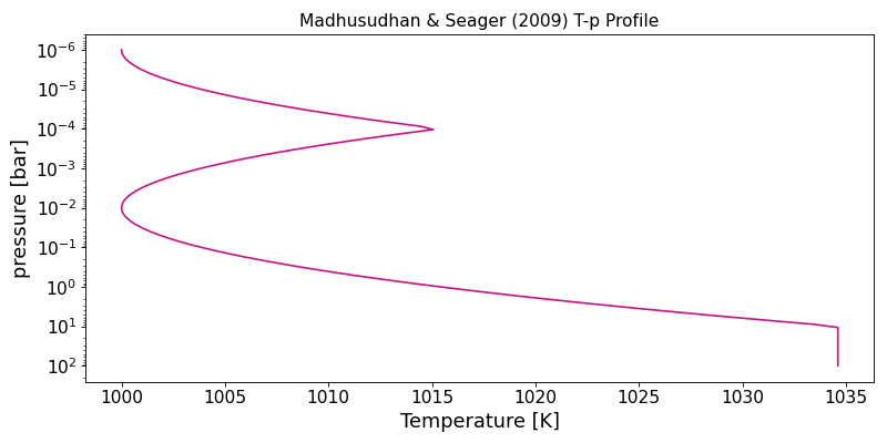
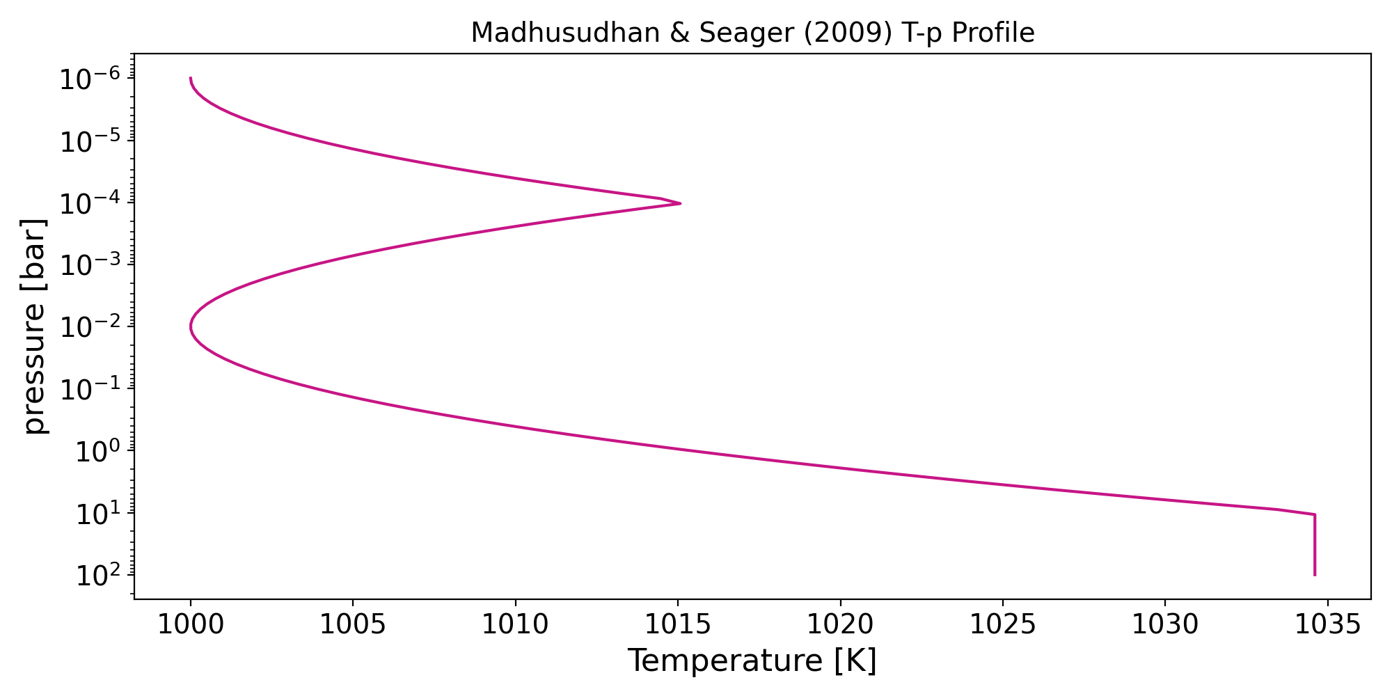
Madhusudhan & Seager (2009)#
The Madhusudhan & Seager (2009) profile uses a piecewise polynomial parameterization with multiple pressure nodes, allowing for flexible T-p profiles with thermal inversions.
This scheme divides the atmosphere into three regions defined by pressure boundaries \(P_1\), \(P_2\), and \(P_3\), with each region having its own temperature gradient controlled by slope parameters \(a_1\) and \(a_2\). This flexibility allows the model to capture both standard profiles and strong thermal inversions often seen in hot Jupiters.
Required parameters: \(a_1\), \(a_2\) (polynomial slope coefficients), \(\log_{10} P_1\), \(\log_{10} P_2\), \(\log_{10} P_3\) [bar] (pressure nodes), \(T_{\rm ref}\) [K] (reference temperature at top of atmosphere)
import numpy as np
import matplotlib.pyplot as plt
from exo_skryer.vert_Tp import MandS
from exo_skryer.data_constants import bar

# Create pressure grid
nlev = 100
p_bot = np.log10(100.0)
p_top = np.log10(1e-6)
p_lev = np.logspace(p_bot, p_top, nlev) * bar

# Example parameters
params = {
    "a1": 0.51,
    "a2": 0.51,
    "log_10_P1": -4.0,
    "log_10_P2": -2.0,
    "log_10_P3": 1.0,
    "T_ref": 1000.0
}
T_lev, T_lay = MandS(p_lev, params)

# Plot
fig, ax = plt.subplots(figsize=(10, 5))
ax.semilogy(T_lev, p_lev/bar, c='mediumvioletred')
ax.set_xlabel('Temperature [K]', fontsize=16)
ax.set_ylabel('pressure [bar]', fontsize=16)
ax.set_title('Madhusudhan & Seager (2009) T-p Profile', fontsize=14)
ax.tick_params(labelsize=14)
ax.invert_yaxis()
plt.tight_layout()
(Source code, png, hires.png, pdf, svg)

Example YAML Configuration:
physics:
  vert_Tp: MandS

params:
  - { name: a1, dist: uniform, low: -2.0, high: 2.0, transform: logit, init: 0.5 }
  - { name: a2, dist: uniform, low: -2.0, high: 2.0, transform: logit, init: -0.4 }
  - { name: log_10_P1, dist: uniform, low: -4, high: 1, transform: logit, init: -2 }
  - { name: log_10_P2, dist: uniform, low: -4, high: 1, transform: logit, init: -0.5 }
  - { name: log_10_P3, dist: uniform, low: -4, high: 2, transform: logit, init: 1 }
  - { name: T_ref, dist: uniform, low: 500.0, high: 3000.0, transform: logit, init: 800.0 }
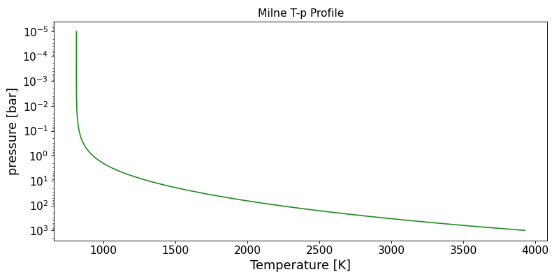
Milne#
A Milne T-p profile is a classic analytical radiative-equilibrium (RE) solution for a grey opacity atmosphere with only an internal heat flux source.
where \(T_{\rm int}\) [K] is the internal (effective) temperature, \(\tau\) the vertical optical depth, \(q(\tau)\) the classic Hopf function solution, that varies between \(q_{\infty} \approx 0.71\) at \(\tau \rightarrow \infty\) and \(q_{0} \approx 1/\sqrt{3}\) at \(\tau \rightarrow 0\).
Required parameters: \(T_{\rm int}\) [K], \(\log_{10}g\) [cm s-2], \(\log_{10} \kappa_{\rm ir}\) [cm2 g-1]
import numpy as np
import matplotlib.pyplot as plt
from exo_skryer.vert_Tp import Milne
from exo_skryer.data_constants import bar

# Create pressure grid
nlev = 100
p_bot = np.log10(1000.0)
p_top = np.log10(1e-5)
p_lev = np.logspace(p_bot, p_top, nlev) * bar

# Example parameters for a brown dwarf
params = {
    "T_int": 1000.0,
    "log_10_g": 4.5,
    "log_10_k_ir": -2.0
}
T_lev, T_lay = Milne(p_lev, params)

# Plot
fig, ax = plt.subplots(figsize=(10, 5))
ax.semilogy(T_lev, p_lev/bar, c='forestgreen')
ax.set_xlabel('Temperature [K]', fontsize=16)
ax.set_ylabel('pressure [bar]', fontsize=16)
ax.set_title('Milne T-p Profile', fontsize=14)
ax.tick_params(labelsize=14)
ax.invert_yaxis()
plt.tight_layout()
(Source code, png, hires.png, pdf, svg)

Example YAML Configuration:
physics:
  vert_Tp: Milne

params:
  - { name: log_10_g, dist: uniform, low: 4.0, high: 5.5, transform: logit, init: 5.0 }
  - { name: T_int, dist: uniform, low: 500.0, high: 1500.0, transform: logit, init: 1000.0 }
  - { name: log_10_k_ir, dist: uniform, low: -6, high: 6, transform: logit, init: -2 }
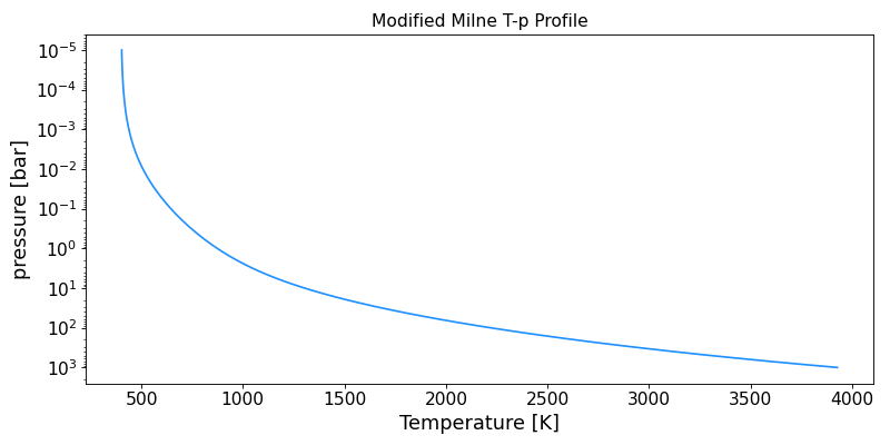
Modified Milne#
The “Modified Milne” profile extends the standard Milne solution to one that smoothly varies from a skin temperature at zero optical depth to the classic Milne solution at high optical depth. It does this by creating a modified Hopf function with a stretched exponential transition following:
where \(T_{\rm int}\) [K] is the internal (effective) temperature, \(\tau\) the vertical optical depth, \(q_{\infty} \approx 0.71\), \(\beta\) is a stretching exponential parameter, which is shallower than exponential for \(\beta < 1\) and steeper when \(\beta > 1\), \(p_{\rm t}\) [bar] the transition region between \(q_{\infty}\) and \(q_{0}\) and \(T_{\rm skin}\) [K] the skin temperature (temperature at zero optical depth). This allows much greater flexibility than the classic Milne solution, and the ability to closely mimic the stucture of (cloud free) non-grey radiative-convective-equilibrium (RCE) models.
Required parameters: \(T_{\rm int}\) [K], \(T_{\rm ratio}\), \(\log_{10}g\) [cm s-2], \(\log_{10} \kappa_{\rm ir}\) [cm2 g-1], \(\log_{10} p_{\rm t}\) [bar], \(\beta\)
import numpy as np
import matplotlib.pyplot as plt
from exo_skryer.vert_Tp import Modified_Milne
from exo_skryer.data_constants import bar

# Create pressure grid
nlev = 100
p_bot = np.log10(1000.0)
p_top = np.log10(1e-5)
p_lev = np.logspace(p_bot, p_top, nlev) * bar

# Example parameters
params = {
    "T_int": 1000.0,
    "T_ratio": 0.4,
    "log_10_g": 4.5,
    "log_10_k_ir": -2.0,
    "log_10_p_t": 0.0,
    "beta": 0.55
}
T_lev, T_lay = Modified_Milne(p_lev, params)

# Plot
fig, ax = plt.subplots(figsize=(10, 5))
ax.semilogy(T_lev, p_lev/bar, c='dodgerblue')
ax.set_xlabel('Temperature [K]', fontsize=16)
ax.set_ylabel('pressure [bar]', fontsize=16)
ax.set_title('Modified Milne T-p Profile', fontsize=14)
ax.tick_params(labelsize=14)
ax.invert_yaxis()
plt.tight_layout()
(Source code, png, hires.png, pdf, svg)

YAML Configuration:
physics:
  vert_Tp: Modified_Milne

params:
  - { name: log_10_g, dist: uniform, low: 4.0, high: 5.5, transform: logit, init: 4.5 }
  - { name: T_int, dist: uniform, low: 500.0, high: 1500.0, transform: logit, init: 1000.0 }
  - { name: T_ratio, dist: uniform, low: 0.0, high: 1.0, transform: logit, init: 0.4 }
  - { name: log_10_k_ir, dist: uniform, low: -6, high: 6, transform: logit, init: -2 }
  - { name: log_10_p_t, dist: uniform, low: -3, high: 2, transform: logit, init: 0.0 }
  - { name: beta, dist: uniform, low: 0.3, high: 1.0, transform: logit, init: 0.55 }