Chemistry Schemes#

The vertical chemistry routines calculate the volume mixing ratio (VMR) of each species, as defined as the fraction of the local total number density of the atmosphere.

Exo Skryer provides several vertical chemistry calculation functions in the vert_chem module.

\[X_{i} = \frac{n_{i}}{n_{\rm tot}}\]

Several schemes are included in Exo Skryer, from simple constant profiles to chemical equilibrium to quenching timescale approximation. In many schemes we assume an H₂-He dominated atmosphere, forcing the total VMR to satisfy

\[\sum_{i}X_{i} = 1\]

For table-interpolated chemistry (fastchem_grid_jax), returned species are the mapped active-opacity set, and VMRs are used directly from the CE table without additional renormalization in vert_chem.

Background Gas: H₂ and He Filling#

After all trace-species VMRs \(X_i\) are determined, the remaining fraction of the atmosphere is filled with H₂ and He following the scheme of Welbanks et al. (2021), ensuring \(\sum_i X_i = 1\):

\[X_{\rm H_2} = \frac{1 - \displaystyle\sum_{i,\,i \neq {\rm He,\,H_2}}^{n} X_i} {1 + \dfrac{X_{\rm He}}{X_{\rm H_2}}}, \qquad X_{\rm He} = X_{\rm H_2}\,\frac{X_{\rm He}}{X_{\rm H_2}},\]

where the He to H₂ ratio is fixed at the solar value from Asplund et al. (2021):

\[\frac{X_{\rm He}}{X_{\rm H_2}} = 0.164.\]

Atomic H and Free-Electron Fraction#

For ultra-hot Jupiter atmospheres where H₂ dissociation is significant, the filling scheme can be extended to include atomic H. A H/H₂ VMR ratio is defined as a retrievable quantity

\[f = \frac{X_{\rm H}}{X_{\rm H_2}},\]

with the background filler fraction

\[X_{\rm bg} = 1 - \sum_{i,\,i \neq {\rm He,\,H_2,\,H}}^{n} X_i,\]

and the solar He/H ratio from Asplund et al. (2021):

\[\epsilon_{\rm He} = \frac{{\rm He}}{{\rm H}} = 0.082.\]

Defining \(N_{\rm H}\) as the dimensionless abundance of hydrogen nuclei in the filler,

\[N_{\rm H} = \frac{X_{\rm bg}}{\dfrac{1+f}{2+f} + \epsilon_{\rm He}},\]

the H₂, H, and He VMRs are then

\[X_{\rm H_2} = \frac{N_{\rm H}}{f + 2}, \qquad X_{\rm H} = f\,X_{\rm H_2}, \qquad X_{\rm He} = \epsilon_{\rm He}\,N_{\rm H}.\]

Note that in certain circumstances \(X_{\rm H} > X_{\rm H_2}\), which should be taken into account when setting prior bounds for the H/H₂ ratio.

This scheme is combined with a free-electron number density fraction \(f_{\rm e^-}\) as a separate retrieved parameter,

\[f_{\rm e^-} = \frac{n_{\rm e^-}}{n_{\rm tot}},\]

where \(n_{\rm e^-}\) [cm^-3] is the electron number density and \(n_{\rm tot}\) [cm^-3] the total background gas number density. Together, the H/H₂ and \(f_{\rm e^-}\) parameters enable a consistent recovery of H^- free–free opacity, an important continuum source in ultra-hot Jupiter atmospheres.

params:
  - { name: log_10_H_over_H2, dist: uniform, low: -6, high: 0, transform: logit, init: -3 }
  - { name: log_10_ne_over_ntot, dist: uniform, low: -6, high: 0, transform: logit, init: -4 }

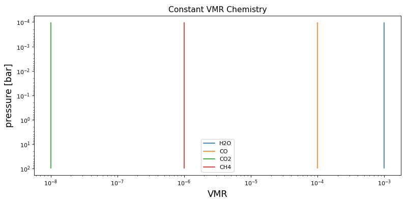
Constant VMR#

The constant VMR profile assumes a constant value for each species as given by the sampled (or delta) parameter, log_10_f_x.

\[X_{i} = X_{\rm const}\]

import numpy as np
import matplotlib.pyplot as plt
from exo_skryer.vert_Tp import Modified_Milne
from exo_skryer.vert_chem import constant_vmr
from exo_skryer.data_constants import bar

nlev = 100
p_bot = np.log10(100.0)
p_top = np.log10(1e-4)
p_lev = np.logspace(p_bot, p_top, nlev) * bar

params_tp = {
    "T_int": 1200.0,
    "T_ratio": 0.333,
    "log_10_g": 4.5,
    "log_10_k_ir": -2.0,
    "log_10_p_t": 0.0,
    "beta": 0.55
}
T_lev, T_lay = Modified_Milne(p_lev, params_tp)
p_lay = (p_lev[1:] - p_lev[:-1]) / np.log(p_lev[1:] / p_lev[:-1])

species_order = ("H2O", "CO", "CO2", "CH4")
chem_kernel = constant_vmr(species_order)
params = {
    "log_10_f_H2O": -3.0,
    "log_10_f_CO": -4.0,
    "log_10_f_CO2": -8.0,
    "log_10_f_CH4": -6.0,
}
vmr_lay = chem_kernel(p_lay, T_lay, params, nlev - 1)

fig, ax = plt.subplots(figsize=(10, 5))
for key in ("H2O", "CO", "CO2", "CH4"):
    if key in vmr_lay:
        ax.semilogy(vmr_lay[key], p_lay / bar, label=key)
ax.set_xlabel("VMR", fontsize=16)
ax.set_ylabel("pressure [bar]", fontsize=16)
ax.set_title("Constant VMR Chemistry", fontsize=14)
ax.legend(fontsize=10)
ax.set_xscale('log')
ax.invert_yaxis()
plt.tight_layout()

(Source code, png, hires.png, pdf, svg)

Example YAML Configuration:

physics:
  vert_chem: constant_vmr

params:
  - { name: log_10_f_H2O, dist: uniform, low: -9, high: -1, transform: logit, init: -3 }
  - { name: log_10_f_CO, dist: uniform, low: -9, high: -1, transform: logit, init: -4 }
  - { name: log_10_f_CO2, dist: uniform, low: -9, high: -1, transform: logit, init: -8 }
  - { name: log_10_f_CH4, dist: uniform, low: -9, high: -1, transform: logit, init: -6 }

Constant VMR (CLR Parameterization)#

constant_vmr_clr parameterizes composition in centered-log-ratio (CLR) space and applies a softmax transform so trace-species plus filler are always non-negative and normalized.

Aliases: constant_clr, clr.

This scheme supports two parameter styles:

native CLR parameters: clr_<species>
standard abundance parameters: log_10_f_<species>

When log_10_f_* is provided, Exo Skryer converts those values to CLR coordinates internally before applying the softmax transform.

Example YAML Configuration:

physics:
  vert_chem: constant_vmr_clr

params:
  - { name: clr_H2O, dist: uniform, low: -12.0, high: 2.0, transform: logit, init: -4.0 }
  - { name: clr_CO,  dist: uniform, low: -12.0, high: 2.0, transform: logit, init: -5.0 }
  - { name: clr_CH4, dist: uniform, low: -12.0, high: 2.0, transform: logit, init: -6.0 }

Alternative (log10 VMR inputs, internally converted to CLR):

physics:
  vert_chem: constant_vmr_clr

params:
  - { name: log_10_f_H2O, dist: uniform, low: -12.0, high: -1.0, transform: logit, init: -4.0 }
  - { name: log_10_f_CO,  dist: uniform, low: -12.0, high: -1.0, transform: logit, init: -5.0 }
  - { name: log_10_f_CH4, dist: uniform, low: -12.0, high: -1.0, transform: logit, init: -6.0 }

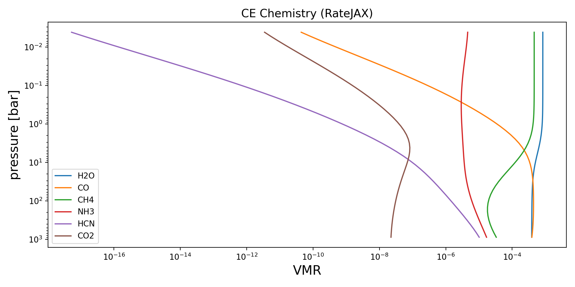
Chemical Equilibrium with rate JAX#

We can also use the semi-analytical chemical equilibrium scheme, Reliable Analytic Thermochemical Equilibrium (rate), from Cubillos et al (2019). This was converted into JAX compatible python from the original python code found on GitHub.

import numpy as np
import matplotlib.pyplot as plt
from pathlib import Path
from exo_skryer.rate_jax import load_nasa9_cache
from exo_skryer.vert_Tp import Modified_Milne
from exo_skryer.vert_chem import CE_rate_jax
from exo_skryer.data_constants import bar

try:
    root = Path(__file__).resolve().parent
except NameError:
    root = Path.cwd().resolve()
for _ in range(5):
    if (root / "NASA9").is_dir():
        break
    root = root.parent
load_nasa9_cache(str(root / "NASA9"))

nlev = 100
p_bot = np.log10(1000.0)
p_top = np.log10(1e-8)
p_lev = np.logspace(p_bot, p_top, nlev) * bar

params_tp = {
    "T_int": 1200.0,
    "T_ratio": 0.333,
    "log_10_g": 4.5,
    "log_10_k_ir": -2.0,
    "log_10_p_t": 0.0,
    "beta": 0.55
}
T_lev, T_lay = Modified_Milne(p_lev, params_tp)
p_lay = (p_lev[1:] - p_lev[:-1]) / np.log(p_lev[1:] / p_lev[:-1])

params = {"M_to_H": 0.0, "C_to_O": 0.55}
vmr_lay = CE_rate_jax(p_lay, T_lay, params, nlev - 1)

fig, ax = plt.subplots(figsize=(10, 5))
for key in ("H2O", "CO", "CH4", "NH3", "HCN", "CO2"):
    if key in vmr_lay:
        ax.semilogy(vmr_lay[key], p_lay / bar, label=key)
ax.set_xlabel("VMR", fontsize=16)
ax.set_ylabel("pressure [bar]", fontsize=16)
ax.set_title("CE Chemistry (RateJAX)", fontsize=14)
ax.legend(fontsize=10)
ax.set_xscale('log')
ax.invert_yaxis()
plt.tight_layout()

(Source code, png, hires.png, pdf, svg)

Example YAML Configuration:

physics:
  vert_chem: CE_rate_jax

params:
  - { name: M_to_H, dist: uniform, low: -1.0, high: 2.0, transform: logit, init: 0.0 }
  - { name: C_to_O, dist: uniform, low: 0.1, high: 1.5, transform: logit, init: 0.55 }

Chemical Equilibrium with FastChem 5D Grid Interpolation#

This backend interpolates a precomputed FastChem grid over (temperature, pressure, M_to_H, C_to_O) using JAX RegularGridInterpolator.

Interpolation is performed in log-space coordinates (log10(T), log10(P), M/H[dex], log10(C/O)) for both legacy linear NPZ grids and log10 NPZ grids. VMR and MMW tables are interpolated in log10 space and converted back to linear values.

The chemistry key is fastchem_grid_jax (aliases: ce_fastchem_grid, fastchem_ce_grid). Legacy ce / fastchem_jax aliases are also supported and route to this backend.

When physics.opac_special enables H^- continuum:

bf requires mapped H- in the CE grid
ff requires mapped H and e- in the CE grid

Initialization raises if required species are missing.

The backend also provides interpolated mean molecular weight to the vert_mu stage via an internal cache key (used automatically by vert_mu: dynamic and vert_mu: auto).

Example YAML Configuration:

physics:
  vert_chem: fastchem_grid_jax

fastchem_grid_jax:
  grid_path: ../../FastChem/fastchem_grid_5d_log10.npz
  solver:
    mode: vmap
  bounds:
    mode: clip
  species_map:
    # Optional per-species mapping override
    # CO: C1O1

Chemical Equilibrium with Atmodeller#

This backend solves equilibrium chemistry with atmodeller using an explicit species network.

The chemistry key is atmodeller.

Example YAML Configuration:

physics:
  vert_chem: atmodeller

atmodeller:
  species_network:
    - H2O_g
    - CO_g
    - CO2_g
    - CH4_g
    - NH3_g
    - H2_g
    - H_g
    - He_g
  solver:
    multistart: 5
    atol: 1.0e-5
    rtol: 1.0e-5
    max_steps: 128

params:
  - { name: M_to_H, dist: uniform, low: -1.0, high: 2.0, transform: logit, init: 0.0 }
  - { name: C_to_O, dist: uniform, low: 0.1, high: 1.5, transform: logit, init: 0.55 }

Chemical Equilibrium with Element Potentials JAX#

This backend solves thermochemical equilibrium from NASA-9 Gibbs free energies using the element-potentials formulation (Lagrange multipliers on element budgets).

The chemistry kernel key is easychem_jax (alias: easychem). Species are configured explicitly in a dedicated YAML block, and all listed species must exist as <species>.txt files in data.nasa9.

Solver mode can be configured:

scan: warm-starts layer-to-layer (typically more robust)
vmap: cold-start parallel solves (often faster on GPU)

Example YAML Configuration:

physics:
  vert_chem: easychem_jax

easychem_jax:
  species: [H2O, CO, CO2, CH4, NH3, HCN, H2, He]
  elements: [H, He, C, N, O]
  e_ref: H
  p0_bar: 1.0
  solver:
    mode: scan
    max_steps: 64
    tol: 1.0e-11
    throw: false
    prefer_chord: true

params:
  - { name: M_to_H, dist: uniform, low: -1.0, high: 2.0, transform: logit, init: 0.0 }
  - { name: C_to_O, dist: uniform, low: 0.1, high: 1.5, transform: logit, init: 0.55 }

Quenching Timescale Approximation#

import numpy as np
import matplotlib.pyplot as plt
from pathlib import Path
from exo_skryer.rate_jax import load_nasa9_cache
from exo_skryer.vert_Tp import Modified_Milne
from exo_skryer.vert_chem import quench_approx
from exo_skryer.data_constants import bar

try:
    root = Path(__file__).resolve().parent
except NameError:
    root = Path.cwd().resolve()
for _ in range(5):
    if (root / "NASA9").is_dir():
        break
    root = root.parent
load_nasa9_cache(str(root / "NASA9"))

nlev = 100
p_bot = np.log10(1000.0)
p_top = np.log10(1e-8)
p_lev = np.logspace(p_bot, p_top, nlev) * bar

params_tp = {
    "T_int": 1200.0,
    "T_ratio": 0.333,
    "log_10_g": 4.5,
    "log_10_k_ir": -2.0,
    "log_10_p_t": 0.0,
    "beta": 0.55
}
T_lev, T_lay = Modified_Milne(p_lev, params_tp)
p_lay = (p_lev[1:] - p_lev[:-1]) / np.log(p_lev[1:] / p_lev[:-1])

params = {"M_to_H": 0.0, "C_to_O": 0.55, "log_10_Kzz": 8.0, "log_10_g": 4.5}
vmr_lay = quench_approx(p_lay, T_lay, params, nlev - 1)

fig, ax = plt.subplots(figsize=(10, 5))
for key in ("H2O", "CO", "CH4", "NH3", "HCN", "CO2"):
    if key in vmr_lay:
        ax.semilogy(vmr_lay[key], p_lay / bar, label=key)
ax.set_xlabel("VMR", fontsize=16)
ax.set_ylabel("pressure [bar]", fontsize=16)
ax.set_title("Quench Approx Chemistry", fontsize=14)
ax.legend(fontsize=10)
ax.set_xscale('log')
ax.invert_yaxis()
plt.tight_layout()

(Source code)

Example YAML Configuration:

physics:
  vert_chem: quench_approx

params:
  - { name: M_to_H, dist: uniform, low: -1.0, high: 2.0, transform: logit, init: 0.0 }
  - { name: C_to_O, dist: uniform, low: 0.1, high: 1.5, transform: logit, init: 0.55 }
  - { name: log_10_Kzz, dist: uniform, low: 5.0, high: 11.0, transform: logit, init: 8.0 }
  - { name: log_10_g, dist: uniform, low: 2.0, high: 4.0, transform: logit, init: 3.0 }

Chemistry Schemes#

Background Gas: H2 and He Filling#

Atomic H and Free-Electron Fraction#

Constant VMR#

Constant VMR (CLR Parameterization)#

Chemical Equilibrium with rate JAX#

Chemical Equilibrium with FastChem 5D Grid Interpolation#

Chemical Equilibrium with Atmodeller#

Chemical Equilibrium with Element Potentials JAX#

Quenching Timescale Approximation#

Background Gas: H₂ and He Filling#