Cloud Vertical Profiles#
Should cloud opacities be required in the retrieval model, first a vertical profile must be defined. Exo Skryer uses the mass mixing ratio, \(q_{\rm c}\) [g g-1], of cloud materials as the basic unit of the vertical cloud profile
where \(\rho_{\rm c}\) [g cm-3] is the condensed cloud mass density and \(\rho_{\rm a}\) [g cm-3] the background atmospheric mass density.
Exo Skryer provides several vertical cloud profile functions in the vert_cloud module.
No Cloud#
A zero cloud profile can be defined, which is useful should custom methods be required that don’t need the cloud mass mixing ratio
Example Plot:
import numpy as np
import matplotlib.pyplot as plt
from exo_skryer.vert_Tp import isothermal
from exo_skryer.vert_cloud import no_cloud
from exo_skryer.data_constants import bar, kb, amu

# Pressure grid (levels → layers)
nlev = 100
p_lev = np.logspace(np.log10(100.0), np.log10(1e-6), nlev) * bar
p_lay = (p_lev[1:] - p_lev[:-1]) / np.log(p_lev[1:] / p_lev[:-1])

# Simple isothermal background state
T_lev, T_lay = isothermal(p_lev, {"T_iso": 1200.0})
mu_lay = np.full_like(T_lay, 2.33)  # amu
nd_lay = p_lay / (kb * T_lay)       # cm^-3
rho_lay = nd_lay * mu_lay * amu     # g cm^-3

q_c_lay = no_cloud(p_lay, T_lay, mu_lay, rho_lay, nd_lay, params={})
q_c_lay = np.asarray(q_c_lay)

fig, ax = plt.subplots(figsize=(9, 4.5))
# Show zero regions on log-x by flooring at a tiny value.
q_floor = 1e-12
q_plot = np.maximum(q_c_lay, q_floor)
ax.loglog(q_plot, p_lay / bar, c="k")
ax.set_xlim(1e-12, 1e-5)
ax.set_xlabel(r"$q_c$ [g g$^{-1}$]", fontsize=14)
ax.set_ylabel("pressure [bar]", fontsize=14)
ax.set_title(r"No Cloud (floored at $10^{-12}$ for log-x)", fontsize=12)
ax.invert_yaxis()
plt.tight_layout()
(Source code, png, hires.png, pdf, svg)

Example YAML Configuration:
physics:
  vert_cloud: no_cloud
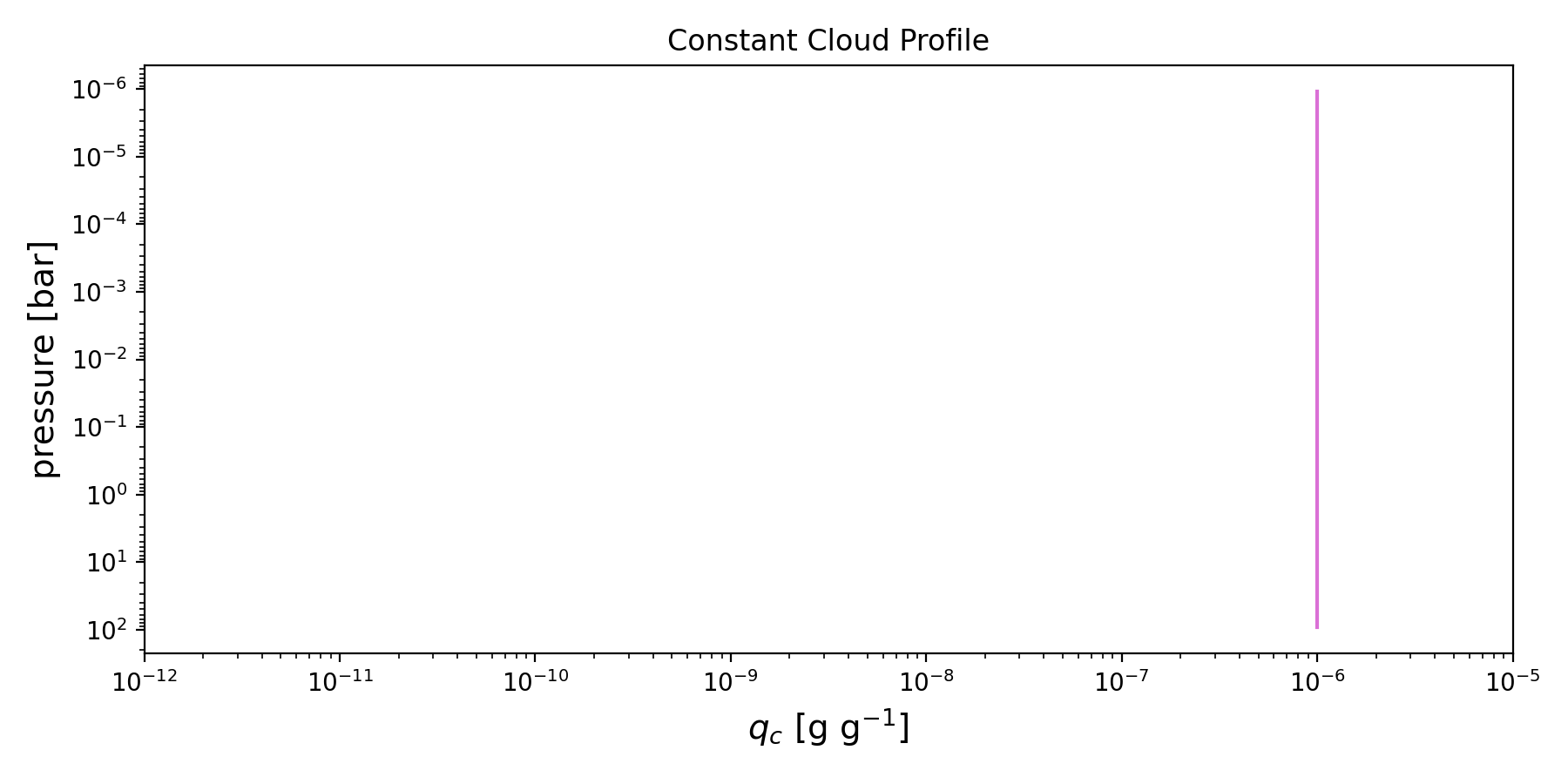
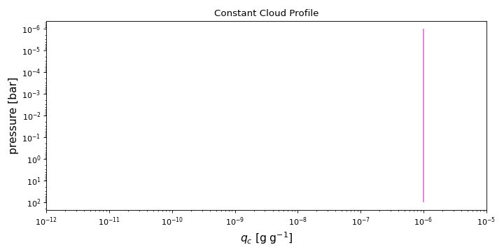
Constant Profile#
A constant (uniform) cloud mass mixing ratio across the entire pressure domain can be given.
Example Plot:
import numpy as np
import matplotlib.pyplot as plt
from exo_skryer.vert_Tp import isothermal
from exo_skryer.vert_cloud import const_profile
from exo_skryer.data_constants import bar, kb, amu

# Create pressure grid
nlev = 100
p_lev = np.logspace(np.log10(100.0), np.log10(1e-6), nlev) * bar
p_lay = (p_lev[1:] - p_lev[:-1]) / np.log(p_lev[1:] / p_lev[:-1])

# Background state (only needed to satisfy kernel signature)
T_lev, T_lay = isothermal(p_lev, {"T_iso": 1200.0})
mu_lay = np.full_like(T_lay, 2.33)  # amu
nd_lay = p_lay / (kb * T_lay)       # cm^-3
rho_lay = nd_lay * mu_lay * amu     # g cm^-3

q_c_lay = const_profile(
    p_lay, T_lay, mu_lay, rho_lay, nd_lay,
    params={"log_10_q_c": -6.0},
)
q_c_lay = np.asarray(q_c_lay)

# Plot
fig, ax = plt.subplots(figsize=(9, 4.5))
ax.loglog(q_c_lay, p_lay / bar, c="orchid")
ax.set_xlim(1e-12, 1e-5)
ax.set_xlabel(r"$q_c$ [g g$^{-1}$]", fontsize=14)
ax.set_ylabel("pressure [bar]", fontsize=14)
ax.set_title("Constant Cloud Profile", fontsize=12)
ax.invert_yaxis()
plt.tight_layout()
(Source code, png, hires.png, pdf, svg)
Example YAML Configuration:
physics:
  vert_cloud: const_profile
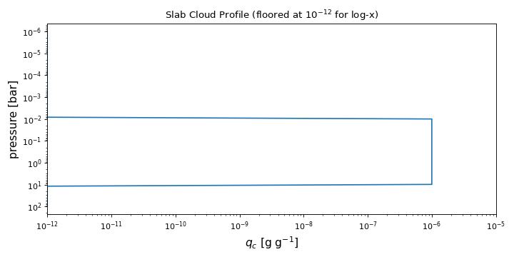
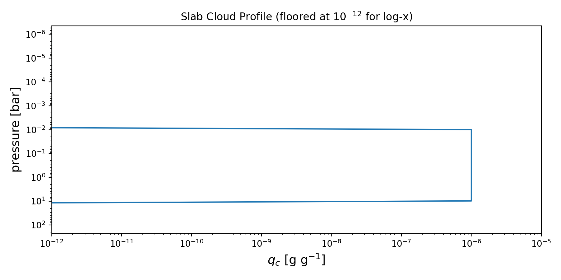
Slab Profile#
A slab profile is defined with a constant \(q_{\rm c}\) between a cloud-top pressure \(p_{\rm top}\) and a bottom pressure \(p_{\rm top} + \Delta p\), where \(\Delta p = 10^{\log_{10} \Delta p}\).
Example YAML Configuration:
physics:
  vert_cloud: slab_profile

params:
  - { name: log_10_q_c, dist: uniform, low: -12, high: -2, transform: logit, init: -6 }
  - { name: log_10_p_top_slab, dist: uniform, low: -6, high: 2, transform: logit, init: -2 }
  - { name: log_10_dp_slab, dist: uniform, low: -2, high: 2, transform: logit, init: 0.5 }
Example Plot:
import numpy as np
import matplotlib.pyplot as plt
from exo_skryer.vert_Tp import isothermal
from exo_skryer.vert_cloud import slab_profile
from exo_skryer.data_constants import bar, kb, amu

nlev = 100
p_lev = np.logspace(np.log10(100.0), np.log10(1e-6), nlev) * bar
p_lay = (p_lev[1:] - p_lev[:-1]) / np.log(p_lev[1:] / p_lev[:-1])

T_lev, T_lay = isothermal(p_lev, {"T_iso": 1200.0})
mu_lay = np.full_like(T_lay, 2.33)
nd_lay = p_lay / (kb * T_lay)
rho_lay = nd_lay * mu_lay * amu

params = {
    "log_10_q_c": -6.0,
    "log_10_p_top_slab": -2.0,  # P_top = 0.01 bar
    "log_10_dp_slab": 1.0,      # Delta_p = 10 bar -> P_bot ~ 10 bar
}
q_c_lay = slab_profile(p_lay, T_lay, mu_lay, rho_lay, nd_lay, params=params)
q_c_lay = np.asarray(q_c_lay)

fig, ax = plt.subplots(figsize=(9, 4.5))
# Log-log plot: floor zeros (outside the slab) to show the zero regions too.
q_floor = 1e-12
q_plot = np.maximum(q_c_lay, q_floor)
ax.loglog(q_plot, p_lay / bar, c="tab:blue")
ax.set_xlim(1e-12, 1e-5)
ax.set_xlabel(r"$q_c$ [g g$^{-1}$]", fontsize=14)
ax.set_ylabel("pressure [bar]", fontsize=14)
ax.set_title(r"Slab Cloud Profile (floored at $10^{-12}$ for log-x)", fontsize=12)
ax.invert_yaxis()
plt.tight_layout()
(Source code, png, hires.png, pdf, svg)

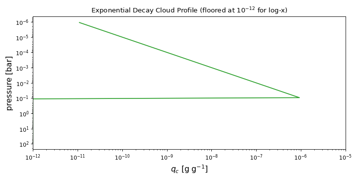
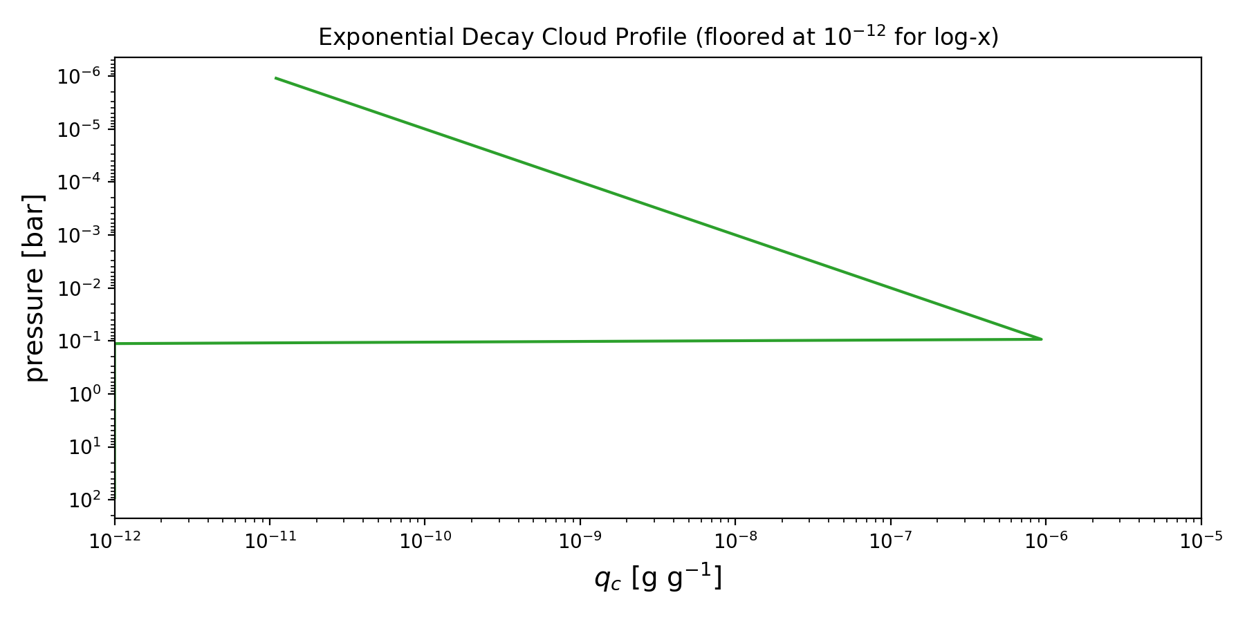
Exponential Decay Profile#
The exponential decay profile reduces the \(q_{\rm c}\) with pressure from a given base value at a base pressure exponentially, given by a decay rate \(\alpha\). Below the base pressure, there is zero cloud.
Example YAML Configuration:
physics:
  vert_cloud: exponential_decay_profile

params:
  - { name: log_10_q_c, dist: uniform, low: -12, high: -2, transform: logit, init: -6 }
  - { name: log_10_alpha_cld, dist: uniform, low: -2, high: 2, transform: logit, init: 0.0 }
  - { name: log_10_p_base, dist: uniform, low: -6, high: 2, transform: logit, init: -1 }
Example Plot:
import numpy as np
import matplotlib.pyplot as plt
from exo_skryer.vert_Tp import isothermal
from exo_skryer.vert_cloud import exponential_decay_profile
from exo_skryer.data_constants import bar, kb, amu

nlev = 100
p_lev = np.logspace(np.log10(100.0), np.log10(1e-6), nlev) * bar
p_lay = (p_lev[1:] - p_lev[:-1]) / np.log(p_lev[1:] / p_lev[:-1])

T_lev, T_lay = isothermal(p_lev, {"T_iso": 1200.0})
mu_lay = np.full_like(T_lay, 2.33)
nd_lay = p_lay / (kb * T_lay)
rho_lay = nd_lay * mu_lay * amu

params = {
    "log_10_q_c": -6.0,
    "log_10_alpha_cld": 0.0,
    "log_10_p_base": -1.0,    # base pressure (bar)
}
q_c_lay = exponential_decay_profile(p_lay, T_lay, mu_lay, rho_lay, nd_lay, params=params)
q_c_lay = np.asarray(q_c_lay)

fig, ax = plt.subplots(figsize=(9, 4.5))
# Log-log plot: floor zeros (below the base) to show the zero regions too.
q_floor = 1e-12
q_plot = np.maximum(q_c_lay, q_floor)
ax.loglog(q_plot, p_lay / bar, c="tab:green")
ax.set_xlim(1e-12, 1e-5)
ax.set_xlabel(r"$q_c$ [g g$^{-1}$]", fontsize=14)
ax.set_ylabel("pressure [bar]", fontsize=14)
ax.set_title(r"Exponential Decay Cloud Profile (floored at $10^{-12}$ for log-x)", fontsize=12)
ax.invert_yaxis()
plt.tight_layout()
(Source code, png, hires.png, pdf, svg)